Session 8. Loops and graphs — Wed 23 Sep

The RAG family, and the index underneath

You have built one kind of RAG. There are several, they are rungs rather than rivals, and each one is worth climbing only when a measurement says so.

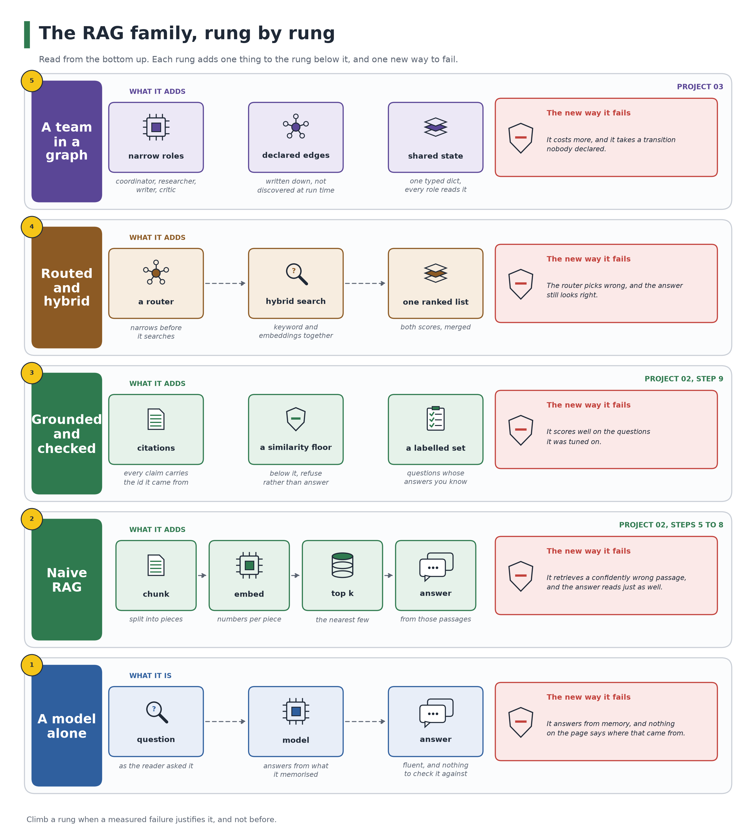
The RAG family as a ladder: a model alone, naive RAG, grounded and checked, routed and hybrid, and a team in a graph, each rung naming what it adds and the new way it fails

The rungs

Rung	What it adds	What it costs	The new way it fails
A model alone	nothing but the prompt	one call	it answers from memory, fluently
Naive RAG	chunk, embed, top k, answer	an index to build and keep	it retrieves a confidently wrong passage
Grounded and checked	citations, a similarity floor, a labelled set	the work of labelling	it scores well on the questions it was tuned on
Routed and hybrid	keyword and embeddings together, a router that narrows first	two retrievers to merge and tune	the router picks wrong, and the answer still looks right
A team in a graph	narrow roles, shared state, declared edges	more model calls per question	a transition nobody declared

Project 02 walked you from naive to grounded. Project 03 is the top rung. You have already met the middle one in session 6, where keyword search and embeddings retrieved different documents for the same question.

Two more names you will hear. Reranking puts a second, slower model over a cheap shortlist, so you retrieve 50 and keep 5. Graph RAG builds a graph of entities at index time and answers from it, which is a different thing from today's agent graph: one is built when you ingest, the other is walked when you ask. If you want the two primary papers, the loop is ReAct (arXiv 2210.03629) and the index-time graph is arXiv 2404.16130.

One honest note. "Agentic RAG" is an umbrella word, not a method with a paper behind it. The methods under it are real and each has its own source. Treat the umbrella as a conversation starter, never as a citation.

Which rung, and when

Your situation	The rung that fits	Why
A handful of documents, and answers you can eyeball	naive	You cannot justify a floor or a labelled set before you have seen it fail.
Anyone else reads the answers	grounded and checked	A citation and a refusal are what make an answer auditable.
Questions arrive in words the documents never use	hybrid	Keyword search misses paraphrases; embeddings miss exact identifiers. Merge both.
The corpus splits cleanly by a field, such as a company or a year	routed	The router narrows before retrieval, and a deterministic one spends no model call.
Stages need different failure policies, or somebody will audit the route	a team in a graph	Each role gets its own prompt, tools and refusal rule, and the state carries the route.

What sits under the index

Retrieval "finds the nearest vectors". How it finds them is a choice, and the choice is a trade between exactness, memory and speed.

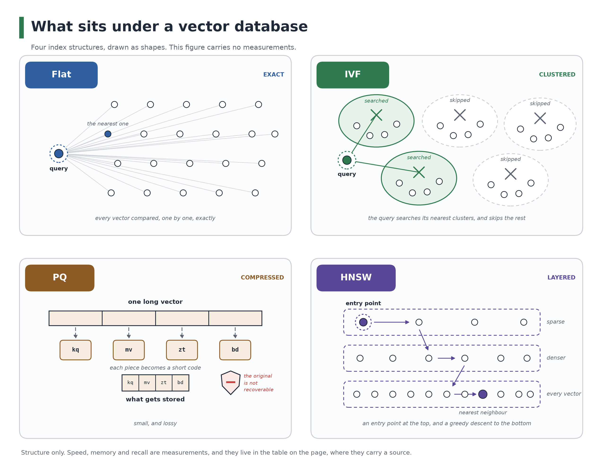
Four index structures drawn as shapes: Flat compares every vector, IVF searches only the nearest clusters, PQ replaces pieces of a vector with short codes, and HNSW descends layers from an entry point to the nearest neighbour

Rather than repeat the speed and memory folklore, here is the one thing the primary source states as arithmetic. These are FAISS's own bytes-per-vector figures, where d is the number of dimensions and M means different things in different rows, as it does in the literature:

Index	Bytes per vector	Exact?
Flat	`4 * d`	yes, brute force
IVF-Flat	`4 * d + 8`	no
PQ	`ceil(M * nbits / 8)`	yes, over compressed codes
IVF-PQ	`ceil(M * nbits / 8) + 8`	no
HNSW	`4 * d + M * 2 * 4`	no

Source: the FAISS index summary and guidelines, read 22 September 2026. The + 8 is the vector id FAISS has to store.

What each one is for, in the sources' own terms:

Flat is the only index that guarantees exact results. No training, no parameters, and search time grows with the data.
IVF splits the space into nlist cells and scans nprobe of them, so roughly nprobe / nlist of the database is compared. It fails when the true neighbour sits in a cell that was not selected.
PQ cuts each vector into M pieces and replaces each piece with a short code. On FAISS's own SIFT benchmark, 512 bytes become 16, which is 32 times smaller, and recall@1 for a 16-byte code measures 0.412 on that codec benchmark. Compression is not free, and that number is what it costs.
IVF-PQ is IVF over PQ-compressed residuals. FAISS calls it the most useful structure for large-scale search, and says compression becomes mandatory somewhere between 10M and 1G vectors per server.
HNSW is layers of a proximity graph: few nodes with long links on top, every node at the bottom. A search enters at the top, walks greedily to a closer neighbour, and descends. FAISS recommends it when memory is not the constraint, and its guidelines put graph indexes below about 1M vectors on a single machine. The vectors can be compressed; the graph cannot.

What our own stack does

We use ChromaDB in projects 01, 02 and 03, so this is not trivia.

Setting	Chroma 1.5.9 default	What it is
`space`	`l2`	squared Euclidean distance, not cosine
`max_neighbors`	16	the `M` of the literature: links per node
`ef_construction`	100	how hard it looks while building
`ef_search`	100	how hard it looks while answering, and the only one you can change later

Measured by creating real collections against the installed chromadb 1.5.9 on 22 September 2026, and cross-checked against Chroma's Rust defaults. Underneath it is still hnswlib.

The gotcha worth ten minutes of your life. The space is l2 even when you attach the default embedding model, whose own declared space is cosine. On vectors that are not normalised, those two metrics do not rank the same way. If you want cosine, ask for it:

collection = client.create_collection(
    "filings",
    configuration={"hnsw": {"space": "cosine", "ef_search": 200}},
)

And the older form is a trap. metadata={"hnsw:search_ef": 55} still works when you create a collection, silently translated and with no warning. On .modify() it is a silent no-op: the metadata key is stored and the index keeps ef_search: 100. Use configuration={"hnsw": {...}} everywhere.

Where HNSW is used, beyond us

Image retrieval, document search, music and product recommendation, and anomaly detection all share one shape: a high-dimensional vector per item, far too many items to compare one by one, and an answer needed while somebody waits. That is the case HNSW is built for. Our eight filings are nowhere near needing it, which is worth saying out loud: at 1,927 passages, a flat scan would be fine. You are running the production index on a toy corpus so that the vocabulary is familiar when the corpus is not.

What this page does not claim

Not "HNSW is O(log n)". The paper derives that under an assumption it then says does not hold, and checks it empirically at four dimensions. At 128 dimensions on 200M vectors the authors themselves report the scaling deviating from a pure logarithm. Sub-linear is safe. Logarithmic is a hedge.
Not "HNSW uses two to four times the memory of IVF". That number circulates widely and we could not source it. The formulas in the table above are what the primary source states, so compute it for your own d and M instead.
No speed table. Speed depends on the dataset, the hardware and the recall you demand. A benchmark without those three named is decoration.

If you want to go deeper

Three short videos, from one vendor's free course. The parameter names are that vendor's spelling (m, ef_construct, hnsw_ef), so read them next to the Chroma names above.

HNSW indexing, 9 minutes. The clearest short answer to why M, ef_construction and ef_search exist. Jump to 4:50, 6:03 and 7:23.
Distance metrics, 3 minutes. Watch it because of the l2 default above. Cosine is at 0:31, Euclidean at 1:26.
Chunking strategies, 11 minutes. The strategies we did not try in project 02: sliding window, recursive, and semantic chunking.